In this quick entry, we show how to format regression output tables in LaTeX and automatically print significance codes (in the form of stars) without any symbols placed a priori.
First of all, one should obtain estimates and standard errors from any statistical package (preferably R, but as long as homicide is considered a crime punishable by incarceration or death, and using SPSS is not, one can use whatever they want – although the author wishes it were the other way about).
Second, one should use regular expressions or any other dark wizardry in order to convert such table into a list of LaTeX control sequences taking two argument each, possible delimited by an ampersand. Here is an example how this can be done by taking raw Excel output (tab-delimited) and running any regex engine on it.
Before:
market  0.0552  0.0055  0.00988 0.00149
ret -1.974  0.0329  -0.767  0.00993
sls -1.31   0.36    -0.342  0.128
age -0.0109 0.0246  -0.00381    0.00663
roa -0.107  0.107   -0.0733 0.0281
Intercept   -0.586  0.138   -0.165  0.036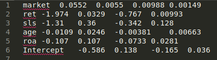
Regular expression for sed:
s/([A-Za-z]+)\t([-0-9.]+)\t([0-9.]+)\t([-0-9.]+)\t([0-9.]+)/\1 & \\coef{\2}{\3} & \\coef{\4}{\5} \\\\/gAfter:
market & \coef{0.0552}{0.0055} & \coef{0.00988}{0.00149} \\
ret & \coef{-1.974}{0.0329} & \coef{-0.767}{0.00993} \\
sls & \coef{-1.31}{0.36} & \coef{-0.342}{0.128} \\
age & \coef{-0.0109}{0.0246} & \coef{-0.00381}{0.00663} \\
roa & \coef{-0.107}{0.107} & \coef{-0.0733}{0.0281} \\
Intercept & \coef{-0.586}{0.138} & \coef{-0.165}{0.036} \\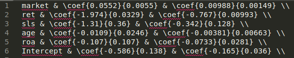
Do not be surprised that now there 3 columns, not 5. Suppose one would like to have the standard error placed beneath the coefficient. Then what?
This is the standard preamble.
\documentclass[11pt, a4paper]{article}
\usepackage[utf8]{inputenc}
\usepackage[T1]{fontenc}
\usepackage{amsmath}
\usepackage{microtype}
\usepackage{booktabs}
\usepackage[british]{babel}
\usepackage{fp}
\newlength\coeflength
\setlength\coeflength{2cm}
Now, it is time to write a command that would typeset a fixed-width box (because all entries in a column have the same width). The basic building block will have 3 arguments: width (optional), estimate (numeric), and standard error (numeric).
\newcommand{\simplestuff}[3][\coeflength]{\parbox[t]{#1}{\hfil$#2$}\parbox[t]{#1}{\hfil$(#3)$}}Now, the stars. The fp package provides facilities to work with fixed-point arithmetic, which is more than enough in our case. Three significance levels—10%, 5%, and 1%—and normal distribution quantiles will be used because this was initially written for applied people in accounting. For asymptotically normal estimators, the critical values can be obtained via the R command qnorm(), e. g. qnorm(1-0.001/2), which should give 3.29 as the critical value for a two-sided t test of significance at 0.1% level.
\newcommand{\coef}[3][\coeflength]{%
\FPset\critsss{2.575829}% 0.995 quantile of the standard normal distribution
\FPset\critss{1.959964}% 0.975 quantile of the standard normal distribution
\FPset\crits{1.644854}% 0.95 quantile of the standard normal distribution
\FPset\coefest{#2}% The first argument is the estimate
\FPset\coefse{#3}% The second argument is the standard error
\FPdiv\zstat{\coefest}{\coefse}% This is the observed t-statistic
\FPabs\zabs{\zstat}% This is its absolute value
\FPiflt\zabs{\crits}\def\kostyrkastar{\relax}\else% Minimising the risk of overwriting an existing command
\FPiflt\zabs{\critss}\def\kostyrkastar{*}\else%
\FPiflt\zabs{\critsss}\def\kostyrkastar{**}\else\def\kostyrkastar{***}%
\fi%
\makebox[#1]{\null\hfill$#2$\kern.1em\rlap{${}^{\kostyrkastar}$}}\makebox[#1]{\null\hfill$(#3)$}%
}
Since hard def’s are used for brevity, in order to minimise the chance that the star-drawing command overwrites any existing one, one should consider using their family name or the name of their pet as a command prefix—above is an example of precautiousness rather than hubris.
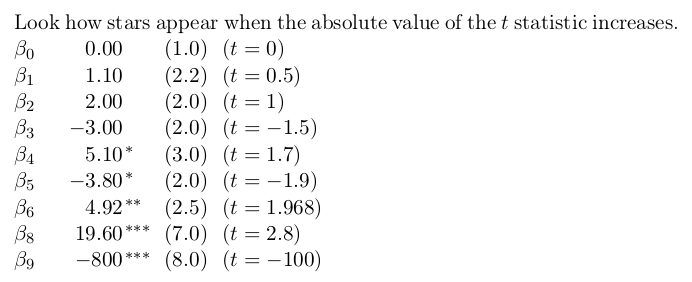
\setlength{\coeflength}{1.5cm}Look how stars appear when the absolute value of the \(t\) statistic increases.
$\beta_0$ \coef{0.00}{1.0} ($t=0$) \par
$\beta_1$ \coef{1.10}{2.2} ($t=0.5$) \par
$\beta_2$ \coef{2.00}{2.0} ($t=1$) \par
$\beta_3$ \coef{-3.00}{2.0} ($t=-1.5$) \par
$\beta_4$ \coef{5.10}{3.0} ($t=1.7$) \par
$\beta_5$ \coef{-3.80}{2.0} ($t = -1.9$) \par
$\beta_6$ \coef{4.92}{2.5} ($t = 1.968$) \par
$\beta_8$ \coef{19.60}{7.0} ($t = 2.8$) \par
$\beta_9$ \coef{-800}{8.0} ($t = -100$)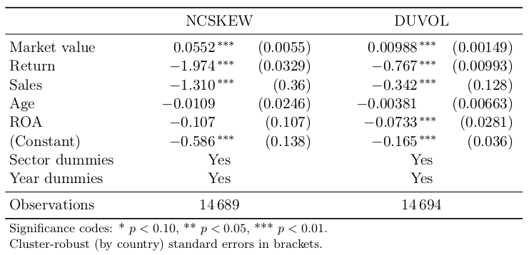
\begin{table}[htbp]
\setlength{\coeflength}{2.2cm}
\setlength{\tabcolsep}{3pt}
\begin{tabular}{lll}
\toprule
& \null\hfill NCSKEW\hfill\null &\null\hfill DUVOL\hfill\null \\
\midrule
Market value & \coef{0.0552}{0.0055} & \coef{0.00988}{0.00149} \\
Return & \coef{-1.974}{0.0329} & \coef{-0.767}{0.00993} \\
Sales & \coef{-1.310}{0.36} & \coef{-0.342}{0.128} \\
Age & \coef{-0.0109}{0.0246} & \coef{-0.00381}{0.00663} \\
ROA & \coef{-0.107}{0.107} & \coef{-0.0733}{0.0281} \\
(Constant) & \coef{-0.586}{0.138} & \coef{-0.165}{0.036} \\
Sector dummies &\null\hfill Yes\hfill\null &\null\hfill Yes\hfill\null \\
Year dummies &\null\hfill Yes\hfill\null &\null\hfill Yes\hfill\null \\
\midrule
Observations &\null\hfill 14\,689\hfill\null &\null\hfill 14\,694\hfill\null \\
\bottomrule
\multicolumn{3}{l}{\footnotesize Significance codes: * $p<0.10$, ** $p<0.05$, *** $p<0.01$.} \\[-.5ex]
\multicolumn{3}{l}{\footnotesize Cluster-robust (by country) standard errors in brackets.} \\
\end{tabular}
\caption{OLS estimates}
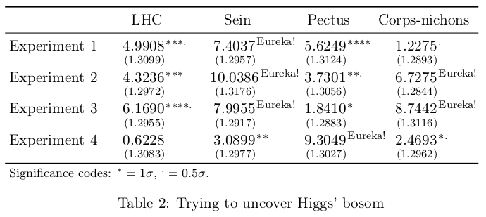
\end{table}If one is working in particle physics and needs to use sigma levels, one can be more creative with their notation. For example, one might need more markers or vertcial placement. This can be achieved in an instant.
\newcommand{\coefnuclear}[3][\coeflength]{%
    \FPset\coefest{#2}%
    \FPset\coefse{#3}%
    \FPdiv\zstat{\coefest}{\coefse}%
    \FPabs\zabs{\zstat}%
    \FPiflt\zabs{0.5}\def\mystar{\relax}\else\FPiflt\zabs{1}\def\mystar{.}\else%
    \FPiflt\zabs{1.5}\def\mystar{*}\else\FPiflt\zabs{2}\def\mystar{*.}\else%
    \FPiflt\zabs{2.5}\def\mystar{**}\else\FPiflt\zabs{3}\def\mystar{**.}\else%
    \FPiflt\zabs{3.5}\def\mystar{***}\else\FPiflt\zabs{4}\def\mystar{***.}\else%
    \FPiflt\zabs{4.5}\def\mystar{****}\else\FPiflt\zabs{5}\def\mystar{****.}\else
    \def\mystar{\text{Eureka!}}\fi%
    \parbox[t]{#1}{\hfil$#2$\kern.1em\rlap{${}^{\mystar}$}\\%
    \null\hfil\scriptsize$(#3)$}
}
\begin{table}[htbp]
    \setlength{\coeflength}{2cm}
    \setlength{\tabcolsep}{3pt}
    \begin{tabular}{lllll}
        \toprule
        & \null\hfill LHC\hfill\null & \null\hfill Sein\hfill\null & \null\hfill Pectus\hfill\null & \null\hfill Corps-nichons \hfill\null\\
        \midrule
        Experiment 1 & \coefnuclear{4.9908}{1.3099} & \coefnuclear{7.4037}{1.2957} & \coefnuclear{5.6249}{1.3124} & \coefnuclear{1.2275}{1.2893} \\[2ex]
        Experiment 2 & \coefnuclear{4.3236}{1.2972} & \coefnuclear{10.0386}{1.3176} & \coefnuclear{3.7301}{1.3056} & \coefnuclear{6.7275}{1.2844} \\[2ex]
        Experiment 3 & \coefnuclear{6.1690}{1.2955} & \coefnuclear{7.9955}{1.2917} & \coefnuclear{1.8410}{1.2883} & \coefnuclear{8.7442}{1.3116} \\[2ex]
        Experiment 4 & \coefnuclear{0.6228}{1.3083} & \coefnuclear{3.0899}{1.2977} & \coefnuclear{9.3049}{1.3027} & \coefnuclear{2.4693}{1.2962} \\
        \bottomrule
        \multicolumn{3}{l}{\footnotesize Significance codes: ${}^* = 1\sigma$, ${}^. = 0.5\sigma$.} \\
    \end{tabular}
    \caption{Trying to uncover Higgs' bosom}
\end{table}
One can change the placement of \hfill and \null to change the alignment. It is, however, a very delicate matter, and good alignment differs from table to table since sometimes, the decimal separator should serve as the pivot. A good (but rather restrictive in real world) idea would be using the same number of digits for all table entries.
Another good example would be using bootstrapped percentile confidence intervals and checking whether zero is inside it or not. One can supply multiple intervals. Making that kind of output is extremely easy if one uses boot package. However, examples of such style in real scientific journals are virtually unseen—because either their typesetters have not read this entry (yet) and are blissfully unaware of this method, or this sort of acrobatics is not deemed æsthetically pleasing or practical.
\newcommand{\coefbootci}[4][\coeflength]{%
    \FPset\coefest{#2}%
    \FPset\coeflb{#3}%
    \FPset\coefub{#4}%
    \parbox[t]{#1}{$#2$\kern0.5em$[#3\hfill%
        \FPiflt\coeflb{0}\FPifgt\coefub{0}\relax\else**\fi%%
        \hfill#4]$}%
}
\coefbootci[4cm]{0.034}{-0.01}{0.09} \par
\coefbootci[4cm]{3.511}{2.048}{5.194}
It is possible to make any formatting aspect adjustable. The last example shows how to make coefficients significant at 5% bold.
\newcommand{\coefbold}[2]{%
    \FPset\coefest{#1}%
    \FPset\coefse{#2}%
    \FPdiv\zstat{\coefest}{\coefse}%
    \FPabs\zabs{\zstat}%
    \FPiflt\zabs{2}\ensuremath{#1}\else\ensuremath{\mathbf{#1}}\fi%
}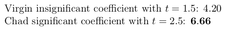
Virgin insignificant coefficient with $t=1.5$: \coefbold{4.20}{2.8} \par
Chad significant coefficient with $t=2.5$: \coefbold{6.66}{2.664}
P.S. In no way is this entry published in order to promote hacking p-values or abusing the data and/or methodology in order to get a sweet succulent p-value that is less than 0.05. Researchers are encouraged to avoid such filthy terms as ‘a convincing trend towards significance’ and other ones, and honestly provide the results as is, using asymptotic refinement via bootstrap, or empirical-likelihood-based with proper calibration, or, in small samples with limited-value variables, exact values for non-parametric small-sample statistics.