Skew-Student t-distribution implementation in R

Carmen Fernandez and Mark F. J. Steel (1998) proposed a generalised family of skewed distributions with highly desirable properties such as analytical moments and applicability to any well-known symmetrical distribution. In particular, they perform Bayesian inference under skew-Student (skew-t) sampling.

The idea behind this extension is very simple: the left half of the probability density function is stretched, and the right half of the density is shrunk by the same skewness parameter \(\gamma \in (0, +\infty)\). The branches are pasted and rescaled so that the PDF should integrate to unity. In fact, I had previously used the same approach for fitting asymmetrical curves in a (later turned out to be futile and way too optimistic!) futile attempt to estimate the number of COVID cases.

Alexios Ghalanos provides C code for the skew-Student density, CDF, quantile, and pseudo-random number generation with two parameters: degree of freedom \(\nu\) and skewness \(\gamma\) (notation from the article). However, typically, one would like to have a location and a scale parameter. The following code is based on distributions.c from the rugarch 1.5 package and extends it to accept two more parameters. These functions do not require any compilation, and works with the highly optimised base-R t-distribution-related functions.

Since the maximum-likelihood approach typically requires logarithmic densities, the logarithm of the density function is available through an optional argument (false by default). This is handy because \(\log f_X(t) \sim \log(1 + x^2)\), which is numerically stable. The R source for dt(), nmath/dt.c, exponentiates the log-density to obtain the vanilla density; therefore, not exponentiating in the first place is the correct way to calculate the log-density of the t-distribution.

NB. The location \(\mu\) and scale \(\sigma\) directly translate to the mean (if \(\nu>1\) and the integral for the expectation converges) and standard deviation if \(\nu > 2\), just like in the analogous functions fro the normal distribution. By default, the distribution is normalised by a function of the degrees of freedom \(\nu\) and skewness \(\gamma\), which is why, with \(\mu = 0, \sigma=1\), the variance of the distrbution in this *sstd implementation is 1 and not \(\frac{\nu}{\nu-2}\). This is especially useful in conditional variance modelling because the series for conditional standard deviation can be directly plugged into the sd argument without any transformations. However, this creates a limitation: we require \(\nu > 2\) to have finite variance. In case one desires to model heavy-tailed distributions with infinite variances, rewrite the logic related to the variance scaling. Solution: write a mapping between the standard deviation and the inter-quartile range of the \(t\)-distribution for \(\nu > 2\) and transition smoothly the IQR scaling (or any other robust dispersion estimator) when \(\nu \le 2\).

# Skew-Student distribution with custom location and scale
# Original C code by Alexios Ghalanos from rugarch 1.5 (distributions.c)
# base R translation and extension by Andreï V. Kostyrka (2024)
heaviside <- function(x) 0.5*(sign(x) + 1)

studMom <- function(df, skew) { # E(X) & SD(X) of the skew-t distribution
  if (df <= 2) stop("Infinite variance of the skew-t distrib.; use df > 2.")
  frac <- (skew^(2:3) + (-1)^(1:2) / skew^(2:3)) / (skew + 1/skew)
  M1 <- 2 * sqrt(df) / (df - 1) / beta(df/2, 0.5) # E|X| for Student
  M2 <- df / (df - 2) # E(X^2) for Student
  EX  <- M1 * frac[1]
  EX2 <- M2 * frac[2]
  return(c(mean = EX, sd = sqrt(EX2 - EX^2)))
}

rsstd <- function(n, mean = 0, sd = 1, df = 10, skew = 1) {
  w <- skew / (skew + 1/skew)
  z <- runif(n, -w, 1-w)
  xx <- ifelse(z < 0, 1/skew, skew)
  rr <- -abs(rt(n, df = df)) / xx * sign(z)
  m <- studMom(df = df, skew = skew)
  ans <- (rr - m[1]) / m[2]
  return(mean + sd*ans)
}

dsstd <- function(x, mean = 0, sd = 1, df = 10, skew = 1, log = FALSE) {
  gp1g <- skew + 1/skew
  m <- studMom(df = df, skew = skew)
  x <- (x - mean) / sd
  z <- (x * m[2] + m[1])
  xxi <- ifelse(z < 0, skew, 1/skew)
  if (log) {
    log(2 / gp1g) + dt(z*xxi, df = df, log = TRUE) - log(sd) + log(m[2])
  } else {
    2 / gp1g * dt(z*xxi, df = df) / sd * m[2]
  }
}

psstd <- function(q, mean = 0, sd = 1, df = 10, skew = 1) {
  q <- (q - mean) / sd
  gp1g <- skew + 1/skew
  m <- studMom(df = df, skew = skew)
  z <- (q * m[2] + m[1])
  xxi <- ifelse(z < 0, skew, 1/skew)
  return(ifelse(z < 0,     2 / gp1g * pt(z*xxi, df = df) / skew,
                       1 - 2 / gp1g * pt(-z*xxi, df = df) * skew))
}

qsstd <- function(p, mean = 0, sd = 1, df = 10, skew = 1) {
  m <- studMom(df = df, skew = skew)
  z <- p - 1/(1 + skew^2)
  Xi <- skew^sign(z)
  tmp <- 0.5 * (skew + 1/skew) * (heaviside(z) - sign(z) * p) / Xi
  (-sign(z) * qt(tmp, df = df) * Xi - m[1]) / m[2] * sd + mean
}

Now we test the behaviour of this function with some nothing-up-my-sleeve parameters to eliminate any chance that these functions have some hidden bugs that do not manifest themselves because some expressions with the ‘nice’ parameters cancel out magically.

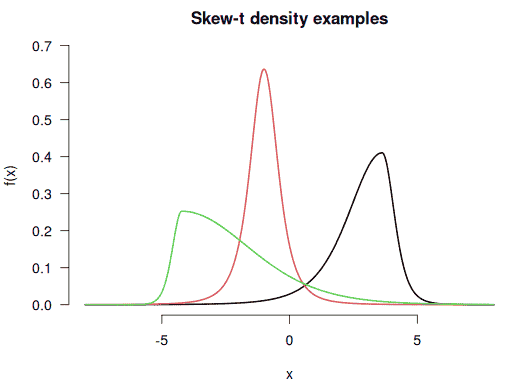
Visualising these custom densities with negative, zero, and positive skewnesses:

f  <- function(x) dsstd(x, mean = 2.8, sd = 1.3, df = 5, skew = 0.6) 
f1 <- function(x) dsstd(x, mean = -1, df = 3, skew = 1)
f2 <- function(x) dsstd(x, mean = -2.2, sd = 2, df = 10, skew = 2.7) 
curve(f(x), from = -8, to = 8, n = 1001, bty = "n", ylim = c(0, 0.7),
      main = "Skew-t density examples", lwd = 2, las = 1)
curve(f1(x), n = 1001, lwd = 2, col = 2, add = TRUE)
curve(f2(x), n = 1001, lwd = 2, col = 3, add = TRUE)

Checking the moments by numerical integration:

integrate(f, -Inf, Inf, rel.tol = 1e-8) # 1
integrate(function(x) x*f(x), -Inf, Inf, rel.tol = 1e-8) # 2.8
integrate(function(x) (x-2.8)^2*f(x), -Inf, Inf, rel.tol = 1e-8) # 1.69=1.3^2
integrate(function(x) ((x-2.8)/1.3)^3*f(x), -Inf, Inf, rel.tol = 1e-8) # < 0

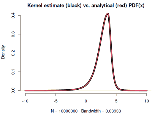
Checking the density and sample moments of the simulated random variable

set.seed(1)
x <- rsstd(1e7, mean = 2.8, sd = 1.3, df = 5, skew = 0.6) # 4 seconds
plot(density(x, from = -10, to = 10), lwd = 5)
curve(f(x), -10, 10, n = 1001, col = 2, lwd = 3, add = TRUE)
round(c(mean(x), sd(x)), 2) # 2.8, 1.3

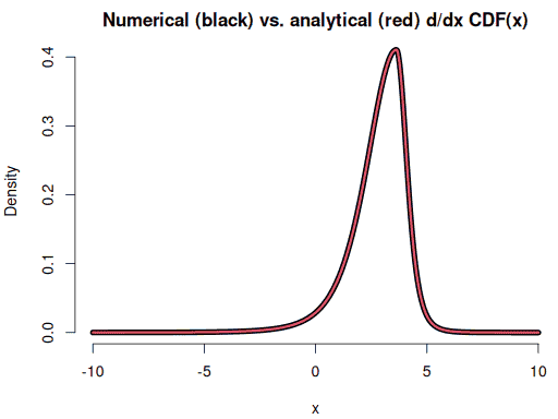
Checking the CDF by comparing its numerical derivative to the PDF:

xseq <- seq(-10, 10, 0.01)
yseq <- psstd(xseq, mean = 2.8, sd = 1.3, df = 5, skew = 0.6)
dyseq <- (psstd(xseq+1e-5, mean = 2.8, sd = 1.3, df = 5, skew = 0.6) - 
          psstd(xseq-1e-5, mean = 2.8, sd = 1.3, df = 5, skew = 0.6)) / (2e-5)
plot(xseq, yseq, pch = 16, bty = "n", main = "Skew-t CDF",
     xlab = "x", ylab = "P(X < x)")
plot(xseq, dyseq, type = "l", lwd = 7, bty = "n", xlab = "x", ylab = "Density",
     main = "Numerical (black) vs. analytical (red) d/dx CDF(x)")
lines(xseq, f(xseq), col = 2, lwd = 3)

Checking the quantile function: \( F\bigl(F^{-1}(p)\bigr) \) should be \(p\) for \(0 < p < 1\):

pseq <- 1:999/1000
max(abs(psstd(qsstd(pseq, mean = 0.12, sd = 2.1, df = 5, skew = 0.5),
        mean = 0.12, sd = 2.1, df = 5, skew = 0.5) - pseq)) # 4 * machine eps
max(abs(qsstd(psstd(xseq, mean = 0.12, sd = 2.1, df = 5, skew = 0.5),
              mean = 0.12, sd = 2.1, df = 5, skew = 0.5) - xseq)) # 1.5e-11!