Last updated: 2019-05-31.
One might ask a question, “What is it like to try to pick an optimal portfolio and invest in stocks?” Well, here I have prepared some R code that does the following thing:
- Downloads stock data from Yahoo Finance from 2014 for a selection of stocks;
- Puts all stocks together across the maximum set of available dates and nicely imputes missing values using Kalman filter with structural modelling;
- Tries all possible combinations or portfolios (as many as possible, using Halton pseudo-random low-discrepancy sequences, doing many iterations and saving the best result from every iteration to save memory);
- Creates amazing colourful plots for subsequent analysis;
- Returns statistics for equally weighted portfolios, max-return under equally weighted risk, min-risk under equally weighted return, and maximum Sharpe ratio (for simplicity, the ratio of returns to risk, assuming there is no risk-free asset);
- Tests these 4 portfolios out of sample for 1 year (“if one started trading one year ago, what would one have obtained”).
Two sets of stocks were chosen: most lucrative U.S. companies and most lucrative Russian companies. This is what one gets if one chooses 13 top U.S. companies:
library(BatchGetSymbols)
library(zoo)
library(imputeTS) # For imputation
library(randtoolbox) # For Sobel sampling
library(parallel)
# http://fortune.com/2017/06/07/fortune-500-companies-profit-apple-berkshire-hathaway/
# https://www.swiftpassportservices.com/blog/profitable-companies-russia/
syms <- c("GOOG", "AAPL", "JPM", "BRK-A", "WFC", "MCD", "BAC", "MSFT", "AMZN", "JNJ", "C", "MO", "GE")
symnames <- c("Google", "Apple", "J.P. Morgan", "Berkshire Hathaway", "Wells Fargo", "McDonald's",
"Bank of America", "Microsoft", "Amazon", "Johnson and Johnson", "Citigroup", "Altria group", "General Electric")
cat("Calculating optimal portfolio for US stocks\n")
# syms <- c("SGTZY", "ROSN.ME", "OGZPY", "LUKOY", "SBRCY", "TRNFP.ME", "NILSY", "ALRS.ME", "YNDX")
# symnames <- c("SurgutNefteGas", "RosNeft", "GazProm", "LukOil", "SberBank", "TransNeft",
# "Norilsk Nickel", "Alrosa", "Yandex")
# cat("Calculating optimal portfolio for Russian stocks\n")
first.date <- as.Date("2014-01-01")
last.date <- as.Date("2018-08-01")
end.ins <- as.Date("2017-08-01")
dat <- BatchGetSymbols(tickers = syms, first.date = first.date, last.date = last.date)
allt <- dat$df.tickers
allt <- allt[!is.na(allt$price.adjusted), ]
dates <- sort(unique(allt$ref.date))
prices <- data.frame(dates)
prices[, 2:(length(syms)+1)] <- NA
colnames(prices)[2:(length(syms)+1)] <- syms
for (i in syms) {
datesi <- allt$ref.date[as.character(allt$ticker)==i]
pricesi <- allt$price.adjusted[as.character(allt$ticker)==i]
prices[match(datesi, dates), i] <- pricesi
prices[, i] <- zoo(prices[, i], order.by = prices$dates)
prices[, i] <- na.kalman(prices[, i])
}
prices2 <- prices
prices[,1] <- NULL
co <- rainbow(length(syms), end=0.75)
png("1-relative-prices.png", 700, 400, type="cairo")
plot(prices[,1]/mean(prices[,1]), col=co[1], lwd=1.5, main="Prices divided by their in-sample mean", xlab="Time", ylab="Ratio")
for (i in 2:length(syms)) {
lines(prices[,i]/mean(prices[,i]), col=co[i])
}
legend("topleft", syms, col=co, lwd=1)
dev.off()
rs <- data.frame(rep(NA, nrow(prices)-1))
for (i in syms) {
rs[, i] <- diff(log(prices[, i]))
}
rs[,1] <- NULL
w0 <- rep(1/length(syms), length(syms))
names(w0) <- syms
rmean <- zoo(as.numeric(as.matrix(rs) %*% w0), order.by = time(rs[,1]))
a <- table(as.numeric(format(time(rmean), "%Y")))
daysperyear <- mean(a[1:(length(a)-1)]) # Because the last year is incomplete
rsfull <- rs # Full sample
rs <- rs[time(rs[,1]) <= end.ins, ] # Training sample
rsnew <- rsfull[time(rsfull[,1]) > end.ins, ] # Test sample
meanrs <- colMeans(rs)
covrs <- cov(rs)
musigma <- function(w) {
mu <- sum(meanrs * w)*daysperyear
s <- sqrt((t(w) %*% covrs %*% w) * daysperyear)
return(c(mu=mu, sigma=s, ratio=mu/s))
}
m0 <- musigma(w0)
num.workers <- if (.Platform$OS.type=="windows") 1 else detectCores()
MC <- 108000
iters <- 100
cc <- 150 # How many colours
cols <- rainbow(cc, end = 0.75)
sharpecuts <- seq(-0.1, 1.5, length.out = cc)
png("2-portfolios.png", 700, 600, type="cairo")
# First iteration
cat("Calculating", MC, "portfolios for the first time.\n")
ws <- halton(MC, length(syms), init=TRUE)
ws <- ws/rowSums(ws)
colnames(ws) <- syms
res <- mclapply(1:MC, function(i) musigma(ws[i, ]), mc.cores = num.workers)
res <- as.data.frame(matrix(unlist(res, use.names = FALSE), nrow=MC, byrow = TRUE))
colnames(res) <- c("mean", "sd", "ratio")
prcmu0 <- ecdf(res$mean)(m0[1]) # Which quantile is the mean
prcsd0 <- ecdf(res$sd)(m0[2]) # Which quantile is the sd
qmplus <- quantile(res$mean, prcmu0+0.005)
qmminus <- quantile(res$mean, prcmu0-0.005)
qsplus <- quantile(res$sd, prcsd0+0.005)
qsminus <- quantile(res$sd, prcsd0-0.005)
meanvicinity <- which(res$mean < qmplus & res$mean > qmminus)
sdvicinity <- which(res$sd < qsplus & res$sd > qsminus)
plot(res[,2:1], pch=16, col=cols[as.numeric(cut(res$ratio, breaks = sharpecuts))],
xlim=range(res$sd)+c(-0.03, 0.03), ylim=pmax(range(res$mean)+c(-0.03, 0.03), c(0, -10)),
main="Risk and return for various portfolios", xlab="Annualised volatility", ylab="Annualised log-return")
sharpes <- mus <- sds <- array(NA, dim=c(iters+1, length(syms)))
sharpes[1, ] <- ws[which.max(res$ratio), ]
mus[1, ] <- ws[which(res$mean == max(res$mean[sdvicinity])), ]
sds[1, ] <- ws[which(res$sd == min(res$sd[meanvicinity])), ]
pairsm <- pairss <- array(NA, dim=c(iters+1, 3))
pairsm[1, ] <- res$mean[c(which.max(res$ratio), which(res$mean == max(res$mean[sdvicinity])), which(res$sd == min(res$sd[meanvicinity])))]
pairss[1, ] <- res$sd[c(which.max(res$ratio), which(res$mean == max(res$mean[sdvicinity])), which(res$sd == min(res$sd[meanvicinity])))]
for (i in 1:iters) {
cat("Calculating", MC, "portfolios, iteration", i, "out of", iters, "\n")
# ws <- sobol(MC, length(syms), scrambling = 1, init=FALSE) # There is a bug in randtoolbox: it starts returning numbers outside [0, 1]
ws <- halton(MC, length(syms), init=FALSE)
ws <- ws/rowSums(ws)
colnames(ws) <- syms
res <- mclapply(1:MC, function(i) musigma(ws[i, ]), mc.cores = num.workers)
res <- as.data.frame(matrix(unlist(res, use.names = FALSE), nrow=MC, byrow = TRUE))
colnames(res) <- c("mean", "sd", "ratio")
meanvicinity <- which(res$mean < qmplus & res$mean > qmminus)
sdvicinity <- which(res$sd < qsplus & res$sd > qsminus)
maxsh <- which.max(res$ratio)
maxm <- which(res$mean == max(res$mean[sdvicinity]))
minsd <- which(res$sd == min(res$sd[meanvicinity]))
sharpes[i+1, ] <- ws[maxsh, ]
mus[i+1, ] <- ws[maxm, ]
sds[i+1, ] <- ws[minsd, ]
pairsm[i+1, ] <- res$mean[c(maxsh, maxm, minsd)]
pairss[i+1, ] <- res$sd[c(maxsh, maxm, minsd)]
points(res[,2:1], pch=16, col=cols[as.numeric(cut(res$ratio, breaks = sharpecuts))])
rm(res); gc()
}
points(as.numeric(pairss), as.numeric(pairsm))
sharpems <- apply(sharpes, 1, musigma)
wmaxsharpe <- sharpes[which.max(sharpems[3,]), ]
meanms <- apply(mus, 1, musigma)
wmaxmean <- mus[which.max(meanms[1,]), ] # Maximum returns while SD is the same
sdms <- apply(sds, 1, musigma)
wminsd <- sds[which.min(sdms[2,]), ] # Minimum SD while mean is the same
m1 <- musigma(wmaxsharpe)
m2 <- musigma(wmaxmean)
m3 <- musigma(wminsd)
finalstats <- cbind(rbind(w0, wmaxsharpe, wmaxmean, wminsd), rbind(m0, m1, m2, m3))
rownames(finalstats) <- c("Equal", "MaxSharpe", "MaxReturn", "MinRisk")
colnames(finalstats)[(length(syms)+1):(length(syms)+3)] <- c("RInS", "VInS", "SRInS")
points(m0[2], m0[1], cex=3, pch=16)
points(c(m1[2], m2[2], m3[2]), c(m1[1], m2[1], m3[1]), cex=2, pch=16)
dev.off()
# And now checking these revenues on the test sample
r0 <- zoo(as.numeric(as.matrix(rsnew) %*% w0), order.by = time(rsnew[,1]))
r1 <- zoo(as.numeric(as.matrix(rsnew) %*% wmaxsharpe), order.by = time(rsnew[,1]))
r2 <- zoo(as.numeric(as.matrix(rsnew) %*% wmaxmean), order.by = time(rsnew[,1]))
r3 <- zoo(as.numeric(as.matrix(rsnew) %*% wminsd), order.by = time(rsnew[,1]))
png("3-test-sample-returns.png", 700, 400, type="cairo")
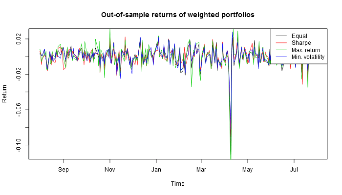
plot(r0, main="Out-of-sample returns of weighted portfolios", ylab="Return", xlab="Time")
lines(r1, col=2)
lines(r2, col=3)
lines(r3, col=4)
legend("topright", c("Equal", "Sharpe", "Max. return", "Min. volatility"), col=1:4, lwd=1)
dev.off()
png("4-test-sample.png", 700, 400, type="cairo")
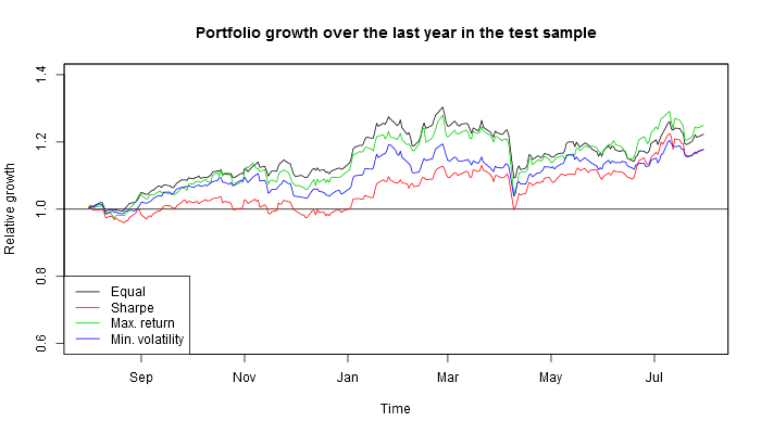
plot(exp(cumsum(r0)), ylim=c(0.6, 1.4), main="Portfolio growth over the last year in the test sample", ylab="Relative growth", xlab="Time")
abline(h=1)
lines(exp(cumsum(r1)), col=2)
lines(exp(cumsum(r2)), col=3)
lines(exp(cumsum(r3)), col=4)
legend("bottomleft", c("Equal", "Sharpe", "Max. return", "Min. volatility"), col=1:4, lwd=1)
dev.off()
finals <- cbind(r0, r1, r2, r3)
meanf <- colMeans(finals)*daysperyear
sdf <- apply(finals, 2, sd)*sqrt(daysperyear)
finalsoos <- cbind(meanf, sdf, meanf/sdf)
colnames(finalsoos) <- c("ROOS", "VOOS", "SRROS")
finalstats <- cbind(finalstats, finalsoos)
colnames(finalstats)[1:length(syms)] <- symnames
library(stargazer)
stargazer(t(finalstats), summary = FALSE, type="html", out="a.html")
write.csv(prices2, "stocks.csv", row.names = FALSE)This is how the 13 U.S. stocks behaved.

This is how 10 million random portfolios behaved (black dots indicate 100 best portfolios under the three criteria; big black dot for the equally weighted portfolio).

These are portfolio weights for U.S. companies with their performance.
| Equal | MaxSharpe | MaxReturn | MinRisk | |
| 0.077 | 0.011 | 0.004 | 0.052 | |
| Apple | 0.077 | 0.132 | 0.128 | 0.105 |
| J.P. Morgan | 0.077 | 0.133 | 0.099 | 0.028 |
| Berkshire Hathaway | 0.077 | 0.019 | 0.040 | 0.170 |
| Wells Fargo | 0.077 | 0.003 | 0.008 | 0.025 |
| McDonald's | 0.077 | 0.164 | 0.148 | 0.192 |
| Bank of America | 0.077 | 0.030 | 0.034 | 0.036 |
| Microsoft | 0.077 | 0.078 | 0.180 | 0.022 |
| Amazon | 0.077 | 0.088 | 0.161 | 0.005 |
| Johnson & Johnson | 0.077 | 0.138 | 0.064 | 0.138 |
| Citigroup | 0.077 | 0.003 | 0.003 | 0.009 |
| Altria group | 0.077 | 0.198 | 0.131 | 0.142 |
| General Electric | 0.077 | 0.003 | 0.001 | 0.078 |
| Return in-sample | 0.145 | 0.179 | 0.190 | 0.145 |
| Risk in-sample | 0.142 | 0.128 | 0.141 | 0.119 |
| Sharpe ratio in-sample | 1.023 | 1.395 | 1.345 | 1.217 |
| Return in 2017.07–2018.06 | 0.135 | 0.163 | 0.241 | 0.053 |
| Risk in 2017.07–2018.06 | 0.144 | 0.134 | 0.146 | 0.130 |
| Sharpe ratio in 2017.07–2018.06 | 0.941 | 1.218 | 1.657 | 0.404 |
This is how these four U.S. portfolios look out of sample.
If one had invested in these four portfolios a year before, this is what one would have harvested by now.
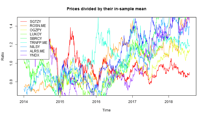
And this is the result for top 9 Russian companies.
This is how the 9 Russian stocks behaved.
This is how 10 million random portfolios behaved (black dots indicate 100 best portfolios under the three criteria; big black dot for the equally weighted portfolio).
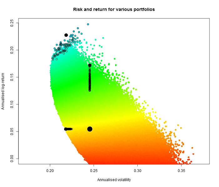
Note that some portfolios can actually yield negative returns, and the volatility is generally higher!
These are portfolio weights for Russian companies with their performance.
| Equal | MaxSharpe | MaxReturn | MinRisk | |
| SurgutNefteGas | 0.111 | 0.005 | 0.009 | 0.175 |
| RosNeft | 0.111 | 0.162 | 0.031 | 0.269 |
| GazProm | 0.111 | 0.012 | 0.068 | 0.067 |
| LukOil | 0.111 | 0.018 | 0.083 | 0.037 |
| SberBank | 0.111 | 0.038 | 0.031 | 0.014 |
| TransNeft | 0.111 | 0.248 | 0.016 | 0.213 |
| Norilsk Nickel | 0.111 | 0.079 | 0.381 | 0.044 |
| Alrosa | 0.111 | 0.413 | 0.358 | 0.049 |
| Yandex | 0.111 | 0.026 | 0.022 | 0.131 |
| Return in-sample | 0.055 | 0.227 | 0.172 | 0.055 |
| Risk in-sample | 0.245 | 0.218 | 0.245 | 0.218 |
| Sharpe ratio in-sample | 0.223 | 1.042 | 0.701 | 0.250 |
| Return in 2017.07–2018.06 | 0.202 | 0.164 | 0.223 | 0.164 |
| Risk in 2017.07–2018.06 | 0.179 | 0.170 | 0.215 | 0.153 |
| Sharpe ratio in 2017.07–2018.06 | 1.129 | 0.965 | 1.039 | 1.067 |
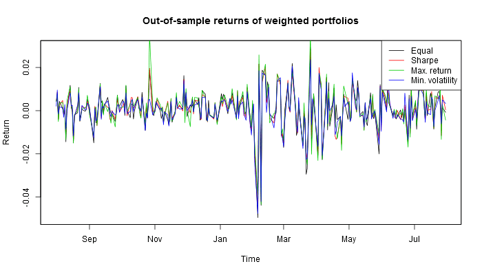
This is how these four Russian portfolios look out of sample.
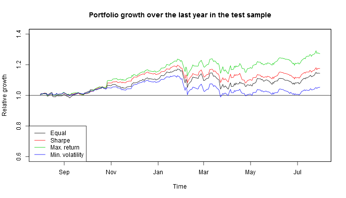
If one had invested in these four portfolios a year before, this is what one would have harvested by now.
So actually if one used this investing strategy based on the information available in mid-2017, by now, depending on the criterion (Sharpe ratio or maximum profitability) they would have earned 14–22% on Russian stocks or 15–17% on American stocks!
[2019-05-31] Update: for high-dimensional problems (hundreds of stocks), many more MC trials are required! One might also want to change the Halton sequence to a random uniform generator (like ws <- matrix(runif(length(syms)*MC), ncol = length(syms))) or a Latin hypercube sampler (lhs).
TODO: constrained optimisation using the best stochastic solution as a starting point.
Why are you still here? Why are you not trading yet?