Any opinions that might be critical of the political system of Russia are justified by the fact that the author was born and grew up in Russia, and retains the right to give opinions, or commentary, or judgement based on his personal experience.
Introduction
Twitter has been known to serve as a news publication machine that drives the attention of mass media and shapes the preferences of voters; a good example of this would be the presidential elections in the USA in 2016 (Kapko, 2016). Presidential candidates were using this medium to communicate to voters directly and express their opinions outside presidential debates. It has been speculated that predictions made based on Twitter data can perform better than those obtained by robocalls or by examining the distribution of lawn signs.
Sometimes, as in the case with Donald Trump, using free-wheeling speech style can be really beneficial because it reassures voters that their candidates speaks what (s)he thinks. Candidates' tweets are news per se, and news agencies can easily get the low-hanging fruit by just re-publishing them and giving their own interpretation. Besides that, Twitter provides an opportunity to engage into a direct dialogue between the candidates and voters via the feature of directed tweets. Celebrities and influential people often respond directly to the candidates, which drives the evolution of voters' views. It has been noted that often it is clear who is writing the tweet: the candidate him/herself or his/her staffers.
As good as it may sound, there are obvious drawbacks to Twitter. First and foremost, it seems almost impossible to fit a meaningful argument within the limit of 140 (now 280) characters. As a result, it causes oversimplification of discourse. Another point is debatable: as soon as something is posted on Twitter, it is impossible to fully withdraw the tweet if someone else has noticed it. This can be both a drawback and a strong point: as soon as lewd material is posted, the poster bears full responsibility for it, and experiences all potential backlash.
Twitter as a predictor for election results has been rigorously analysed by researchers in the past. In fact, such analyses were applied to the 2010 Australian elections (Burgess and Bruns, 2012), 2010 Swedish elections (Larsson and Moe, 2012), 2011 Dutch elections (Sang and Bos, 2012), 2012 USA elections (Wang et al., 2012), 2015 Venezuelan elections (Yang, Macdonald and Ounis, 2017), 2016 USA elections (Bessi and Ferrara, 2016) etc. Some of them are using convolutional neural networks, some of them are applying clever tools to avoid misclassification, but some of them rely on a simple count of words from positive and negative dictionaries. We are going to adopt this simple approach in an attempt to analyse Russian data and evaluate the balance of powers (or lack thereof) in Russia.
In this work, I am using big data (70 000 tweets in total) and big data processing tools (Google Translate API) to investigate the relative popularity of candidates in the Russian presidential election of 2018. The methodology will be similar to that of Bhatia (2015).
Methodology
In this work, I develop a simple method to analyse the sentiment towards election candidates in arbitrary languages using Google Translate. It should be noted that as the moment of writing, Google is offering a free $300 trial for its Cloud API, so the author made use of his free access to the machine translation services. The workflow is as follows:
- Using R and twitteR package, obtain a large number (10 000) tweets mentioning the candidate;
- Break the tweets into small batches (100 tweets per batch separated with triple paragraphs) and write scripts for translation;
- Using Google Cloud Translation API, run the translation scripts and obtain the server response as a JSON object;
- Input the JSON object into R, break it into separate tweets again and clean up the text;
- Count the positive and negative words in those tweets using dictionaries and analyse the distributions.
Obviously, the main drawback of the simple dictionary match is the lack of context. There are examples of why this might return wrong results. Example 1: “Mr. X is going to put an end to corruption!” This author has a positive attitude towards Mr. X, but due to the presence of a negative word (“corruption”), is going to be counted as negative. Example 2: “@newsagency Yes, of course, Mr. Y is going to improve the situation, yeah, like, thousand times!” This is an example of irony; the attitude of this tweet is negative and sceptical, but the simple count will find a positive match (“improve”) and count this tweet as positive. Example 3: “Mr. Z is not honest!”
To counter these three points, an argument should be made. The error from the first category does not change much in terms of emotional attitude; if candidate X is viewed as a corruption fighter, the writer implies that the situation in the country is grave (hence the need to fight), and this negative score should be counted towards the general level of negativity, not just the negativity associated with candidate X. If candidates Y and Z also claim they are going to fight corruption, then all these negative votes will contribute to a fixed proportion of false negatives (say, n%), and the ratio of negative to positive votes should not change. This implies that ratios, not absolute values should be examined. The error from the second category is so semantically complicated that is it improbable that any advanced methods (including machine learning and neural networks) based on pure text analysis are going to detect irony and correctly interpret it in a negative sense. However, the proportion of such tweets is thought to be low, and an advanced user-based analysis is suggested in this case: if a user is generally opposing candidate Y (or is pessimistic in general), then any tweets with positive score about candidate Y should be re-weighted or discarded as “implausible”. The error from the third category, however, can be remedied with the use of multi-layered neural network or contextual analysis algorithms with look-ahead and look-behind: if the word from the “positive” list is preceded by “not”, “no”, “barely” or followed by “my a**” or other similar modifiers, the match should be counted for the “negative” list, and vice versa.
Implementation
Searching for tweets
Assumption 1. During the period from 2018-01-01 to 2018-03-18, any tweet containing the surname of a candidate is meant to be about the candidate, not his namesake.
This assumption allows us to identify tweets about the presidential candidates by a simple search using the name of the candidate. The candidates seem to have quite unique surnames, and almost all media covering people with their surnames are covering namely those people.
Assumption 2. There is no bias in Twitter search results; i. e., Twitter is not being in favour of any candidate, or is not filtering negative search results, or is not affected by spam bots who praise candidates.
This assumption is crucial for the unbiasedness of our results; so far, there have been no signs of Twitter censorship in Russia. However, there might be a population bias: people who are using Twitter can turn out to be younger and more progressive, and therefore, more opposing to the current political leader, Putin. It means that whereas most tweets about Putin on Twitter can come from a minority of political opposition, the majority of Putin voters are budget-depending elderly people and beneficiaries who live in faraway regions without internet access or any desire to express their opinions publicly.
api_key <- "..."
api_secret <- "..."
access_token <- "..."
access_token_secret <- "..."

library(twitteR)
setup_twitter_oauth(api_key, api_secret, access_token, access_token_secret)

find1 <- "Путин"
find2 <- "Бабурин"
find3 <- "Грудинин"
find4 <- "Жириновский"
find5 <- "Собчак"
find6 <- "Сурайкин"
find7 <- "Титов"
find8 <- "Явлинский"
find9 <- "Навальный"
finds <- c(find1, find2, find3, find4, find5, find6, find7, find8, find9)

number <- 10000

tweet1 <- searchTwitter(find1, n=number, lang="ru", since="2018-01-01", until="2018-03-18")
tweet2 <- searchTwitter(find2, n=number, lang="ru", since="2018-01-01", until="2018-03-18")
tweet3 <- searchTwitter(find3, n=number, lang="ru", since="2018-01-01", until="2018-03-18")
tweet4 <- searchTwitter(find4, n=number, lang="ru", since="2018-01-01", until="2018-03-18")
tweet5 <- searchTwitter(find5, n=number, lang="ru", since="2018-01-01", until="2018-03-18")
tweet6 <- searchTwitter(find6, n=number, lang="ru", since="2018-01-01", until="2018-03-18")
tweet7 <- searchTwitter(find7, n=number, lang="ru", since="2018-01-01", until="2018-03-18")
tweet8 <- searchTwitter(find8, n=number, lang="ru", since="2018-01-01", until="2018-03-18")
tweet9 <- searchTwitter(find9, n=number, lang="ru", since="2018-01-01", until="2018-03-18")

save(tweet1, tweet2, tweet3, tweet4, tweet5, tweet6, tweet7, tweet8, tweet9, file="tweets.RData")
Breaking the tweets for translation
A simple snippet of code is suggested below to translate the long and heavy objects on Google Translate. As we know, Google charges API users on a character basis (as of writing, $20 per 1 million characters), with virtually no limit for translation (if the proper quotas are set to be infinite). However, just in order to be sure that the translations are made in time and no information is lost, we broke the messages into blocks of 100 tweets.
byhow <- 100

for (cand in 1:9) {
  texts <- get(paste0("tweet", cand))
  blocks <- ceiling(length(get(paste0("tweet", cand)))/byhow)
  for (i in 1:blocks) {
    sink(paste0("scripts", cand, "/scr", i, ".sh"))
    fr <- byhow*(i-1)+1
    to <- byhow*(i-1)+byhow
    cat('
    curl -s -X POST -H "Content-Type: application/json" \\
    -H "Authorization: Bearer "$(gcloud auth print-access-token) \\
    --data "{
      \'q\': \'
      ')
      if (to > length(texts)) to <- length(texts)
      for (j in fr:to) {
        cat("\n\n\n")
        a <- texts[[j]]$text
        a <- gsub("['\"`]", "", a)
        cat(a)
      }
      cat('
      \',
      \'source\': \'ru\',
      \'target\': \'en\',
      \'format\': \'text\'
    }" "https://translation.googleapis.com/language/translate/v2"

    ')
    sink()
  }

}
Therefore, for each of the nine candidates, it will write out up to 100 script files into a corresponding folder.
Using Google Translate API
Once the script files, titled scr1.sh, ..., scr100.sh are ready, all that remains is run them in series with a time-out (since Google API has a character-per-minute quota).
#!/bin/bash
for i in {1..100}
  do
  echo "Processing tweet file $i of 100"
  ./scr$i.sh > out$i.txt
  sleep 12
done
This script must be run in every folder (1–9), and the translation results will be stored in files out1.txt, ..., out100.txt (or up to the number of tweets divided by 100 if the candidate was not very popular).
Merging the objects into tweet lists
A simple for loop (for 9 candidates, from 1 to the number of output files) is required to merge the data back.
library(jsonlite)

alltrans <- list()

for (cand in 1:9) {
  lf <- list.files(paste0("./scripts", cand, "/"))
  lf <- lf[grep("out", lf)]
  howmany <- length(lf)

  alltrans[[cand]] <- list()

  for (i in 1:howmany) {
    a <- fromJSON(readLines(paste0("scripts", cand, "/out", i, ".txt")))
    a <- a[[1]]$translations$translatedText
    aa <- strsplit(a, "\n\n\n")[[1]]
    aa <- gsub("@ +", "@", aa)
    aa <- gsub("^\n +", "", aa)
    aa <- aa[aa!=""]

    alltrans[[cand]][[i]] <- aa
    if (! i%%10) print(paste0("Candidate ", cand, ": ", i, " out of ", howmany))
  }
}

clean <- function(t) {
  t <- gsub('[[:punct:]]', '', t)
  t <- gsub('[[:cntrl:]]', '', t)
  t <- gsub('\\d+', '', t)
  t <- gsub('[[:digit:]]', '', t)
  t <- gsub('@\\w+', '', t)
  t <- gsub('http\\w+', '', t)
  t <- gsub("^\\s+|\\s+$", "", t)
  t <- gsub('"', '', t)
  t <- strsplit(t,"[ \t]+")
  t <- lapply(t, tolower)
  return(t)
}

alltrans2 <- lapply(alltrans, unlist)

alltrans3 <- lapply(alltrans2, clean)
This clean-up included removing punctuation, control characters, URLs, and digits from the tweets, and then splitting them at spaces or tabs. For matching, conversion to lowercase was used.
Analysing sentiments
First and foremost, we look at the distributions of positive and negative tweet counts for various candidates.
positive <- scan('positive-words.txt', what='character', comment.char=';')
negative <- scan('negative-words.txt', what='character', comment.char=';')

posscore <- function(tweet) {
pos.match <- match(tweet, positive)
pos.match <- !is.na(pos.match)
pos.score <- sum(pos.match)
return(pos.score)
}

negscore <- function(tweet) {
neg.match <- match(tweet, negative)
neg.match <- !is.na(neg.match)
neg.score <- sum(neg.match)
return(neg.score)
}

posscores <- list()
negscores <- list()
for (i in 1:9) {
posscores[[i]] <- unlist(lapply(alltrans3[[i]], posscore))
negscores[[i]] <- unlist(lapply(alltrans3[[i]], negscore))
}

poscounts <- lapply(posscores, table)
negcounts <- lapply(negscores, table)

cols <- rainbow(10)

cairo_pdf("counts1.pdf", 7, 5)
plot(NULL, NULL, xlim=c(0, 6.7), ylim=c(0, 7516), main = "Positive tweet counts for candidates", ylab = "Tweets", xlab="Positive words in a tweet")
for (j in 1:9) {
for (i in 1:length(poscounts[[j]])) {
lines(c(i-1 + (j-1)/10, i-1 + (j-1)/10), c(0, poscounts[[j]][i]), lwd=5, col=cols[j])
}
}
legend("topright", finds, lwd=5, col=cols)
dev.off()

cairo_pdf("counts2.pdf", 7, 5)
plot(NULL, NULL, xlim=c(0, 6.7), ylim=c(0, 7516), main = "Negative tweet counts for candidates", ylab = "Tweets", xlab="Negative words in a tweet")
for (j in 1:9) {
for (i in 1:length(negcounts[[j]])) {
lines(c(i-1 + (j-1)/10, i-1 + (j-1)/10), c(0, negcounts[[j]][i]), lwd=5, col=cols[j])
}
}
legend("topright", finds, lwd=5, col=cols)
dev.off()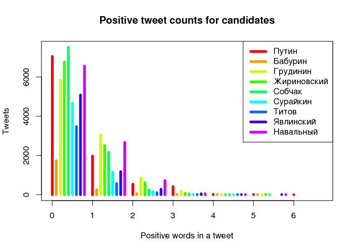
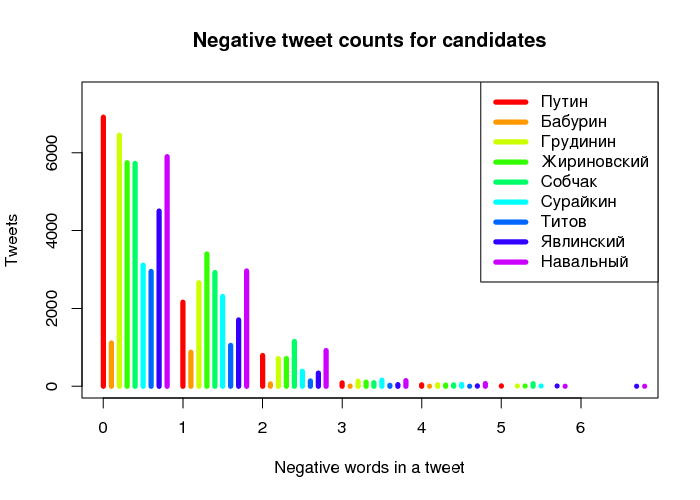
Fig. 1. Distribution of tweets
Since there is no real political competition to Putin (position 1) among the present candidates (positions 2–8), let us pay some attention to his closest political rival who was denied access to the elections, Navalny (position 9). As we can see from Fig. 1, the number of tweets related to Putin and containing 1–2 positive words is smaller than that related to Navalny. At the very same time, paradoxically, the number of tweets related to Putin and containing 1–2 negative words is also smaller than that of Navalny.
totpos <- numeric(9)
totneg <- numeric(9)
for (i in 1:9) {
totpos[i] <- sum(poscounts[[i]] * as.numeric(names(poscounts[[i]])))
totneg[i] <- sum(negcounts[[i]] * as.numeric(names(negcounts[[i]])))
}

# Ordering candidates not alpabetically but as they are in the database
a <- factor(finds)
finds <- factor(a, levels(a)[c(5, 1, 2, 3, 6, 7, 8, 9, 4)])

ratios <- totpos/totneg
ratiosdf <- data.frame(ratio=ratios, name=finds)

library(ggplot2)
p <- ggplot(data=ratiosdf, aes(x=name, y=ratio, fill=name)) + geom_bar(stat="identity") + ylab("Positive/negative ratio") +
theme_minimal() + coord_flip() + scale_x_discrete(limits = rev(levels(ratiosdf$name))) + theme(legend.position="none", axis.title.y=element_blank())
cairo_pdf("ratios.pdf", 8, 7)
plot(p)
dev.off()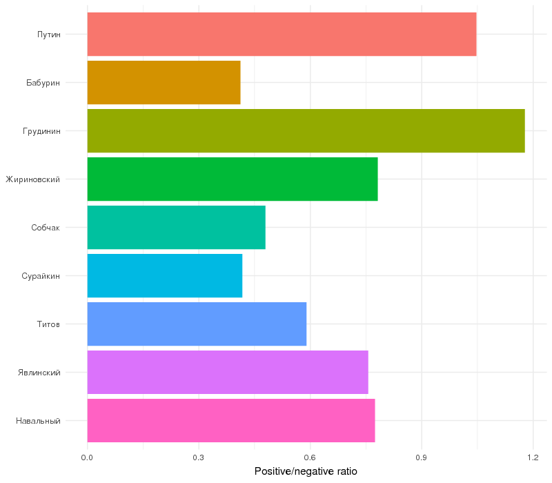
Fig. 2. Tweet sentiment ratios for candidates
It is unsurprising that that the ratio for Navalny, who is known as a fighter against corruption, is lower than that of Putin, despite the fact that there is a substantial number of opposing bloggers, due to the fact that the word “corruption” is negative per se. In general, only one candidate (Grudinin) has this ratio greater or equal to one. This means that tweets containing the names of political leaders are negative in tone in general.
Now we visualise which words were the top positive and top negative for each candidate.
poswords <- function(tweets) {
pmatch <- match(t, positive)
posw <- positive[pmatch]
posw <- posw[!is.na(posw)]
return(posw)
}

negwords <- function(tweets) {
pmatch <- match(t, negative)
negw <- negative[pmatch]
negw <- negw[!is.na(negw)]
return(negw)
}

pdata <- list()
ndata <- list()
for (j in 1:9) {
pdata[[j]] <- ""
ndata[[j]] <- ""
for (t in alltrans3[[j]]) {
pdata[[j]] <- c(poswords(t), pdata[[j]])
ndata[[j]] <- c(negwords(t), ndata[[j]])
}
}

pfreqs <- lapply(pdata, table)
nfreqs <- lapply(ndata, table)

dpfreq <- list()
dnfreq <- list()
for (j in 1:9) {
thresh <- length(alltrans2[[j]])/200
a <- pfreqs[[j]]
a <- a[a>thresh]
b <- nfreqs[[j]]
b <- b[b>thresh]
dpfreq[[j]] <- data.frame(word=as.character(names(a)), freq=as.numeric(a))
dpfreq[[j]]$word <- as.character(dpfreq[[j]]$word)
dnfreq[[j]] <- data.frame(word=as.character(names(b)), freq=as.numeric(b))
dnfreq[[j]]$word <- as.character(dnfreq[[j]]$word)
}

for (j in 1:9) {
p1 <- ggplot(dpfreq[[j]], aes(word, freq)) + geom_bar(stat="identity", fill="lightblue") + theme_bw() +
geom_text(aes(word, freq, label=freq), size=4) + labs(x="Major Positive Words", y="Frequency of Occurence",
title=paste0("Major Positive Words and Occurence for \n", finds[j], ", n = ", length(alltrans2[[j]]))) +
theme(axis.text.x=element_text(angle=90))
p2 <- ggplot(dnfreq[[j]], aes(word, freq)) + geom_bar(stat="identity", fill="pink") + theme_bw() +
geom_text(aes(word, freq, label=freq), size=4) + labs(x="Major Negative Words", y="Frequency of Occurence",
title=paste0("Major Negative Words and Occurence for \n", finds[j], ", n = ", length(alltrans2[[j]]))) +
theme(axis.text.x=element_text(angle=90))
cairo_pdf(paste0("posw", j, ".pdf"),  2+nrow(dpfreq[[j]])/8, 5)
plot(p1)
dev.off()
cairo_pdf(paste0("negw", j, ".pdf"),  2+nrow(dnfreq[[j]])/8, 5)
plot(p2)
dev.off()
}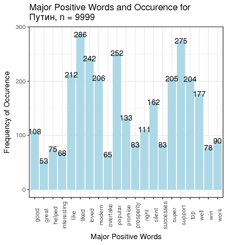
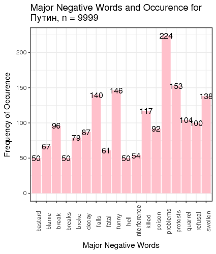
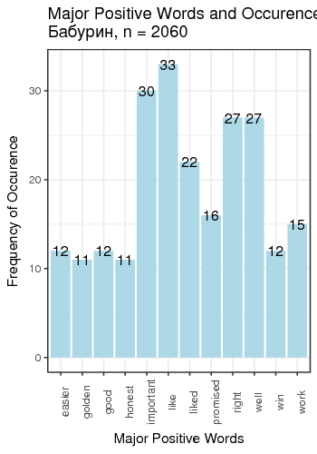
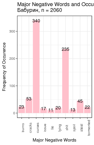
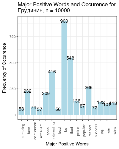
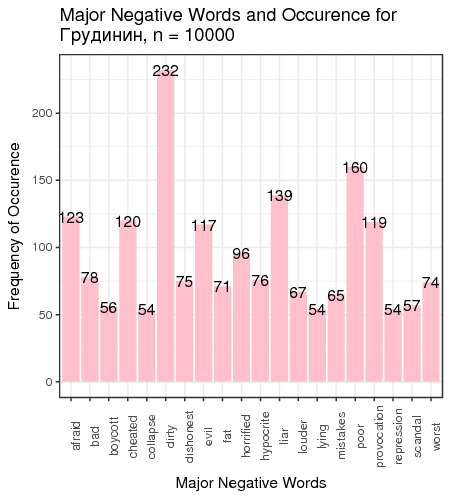
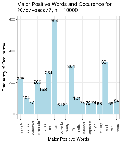
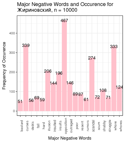
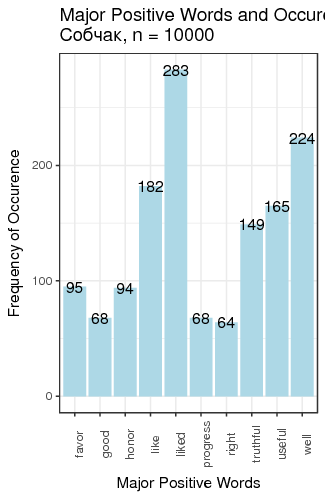
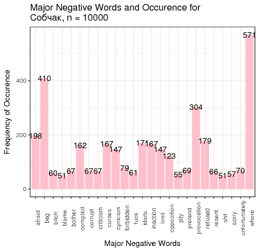
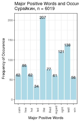
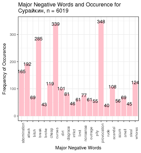
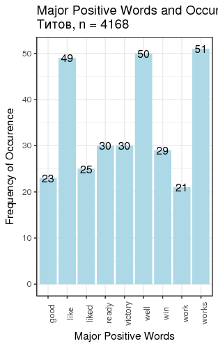
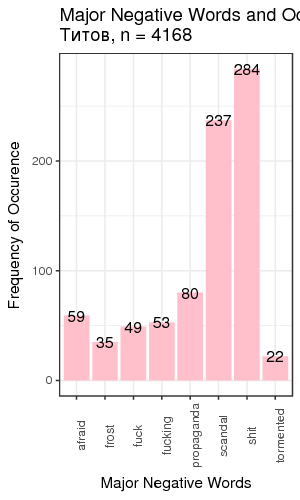
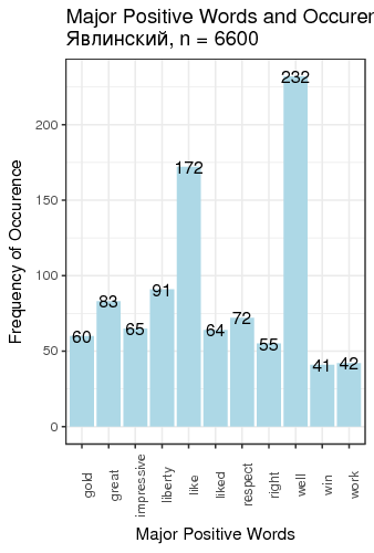
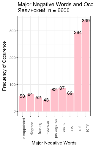
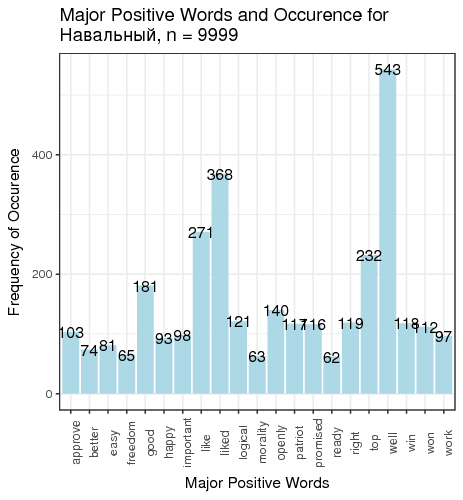
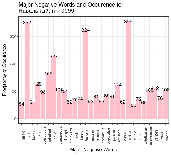
Fig. 3. Most frequent positive and negative words for candidates
We defined “most frequent” words as words whose count exceeded the total number of tweets divided by 200. There is just one small problem: such generic words as “like” and “right”, “well” etc. are on this table. We can remedy that by manually constructing a table of most popular meaningful positive and negative words for candidates (Table 1).
| Candidate | 1st + word | 2nd + word | 1st − word | 2nd − word |
|---|---|---|---|---|
| Putin | support 275 | popular 252 | problems 224 | protests 153 |
| Baburin | important 30 | right 27 | curses 340 | shit 235 |
| Grudinin | interesting 416 | respect 266 | dirty 232 | poor 160 |
| Zhirinovsky | benefit 225 | entertain 206 | curses 339 | whore 333 |
| Sobchak | useful 165 | truthful 149 | whore 571 | beg 410 |
| Surajkin | free 86 | regard 61 | provocation 348 | curses 339 |
| Titov | works 51 | ready 30 | shit 284 | scandal 237 |
| Yavlinsky | liberty 91 | great 83 | sorry 339 | shit 294 |
| Navalny | top 232 | good 181 | strike 355 | boycott 352 |
Table 1. Two most frequent meaningful words for candidates
Conclusions
We can make several conclusions. First, several candidates (Baburin, Surajkin, Titov, Yavlinsky) are so unpopular that they were not mentioned 10 000 times over the course of 2.5 months since the beginning of 2018, which implies that they were added to the list of approved candidates to create the illusion of choice; they cannot compete against the obvious leader of the race. Next, on average, people tweet about politicians when they are discontent with something; it is reflected in the average negative score of tweets, except for Putin and Grudinin. Some politicians (Zhirinovsky, Sobchak) are viewed as politically promiscuous, which is reflected in the word frequency analysis. This all creates the illusion of choice presence, whereas most of the population of Russia does not have access to Twitter, or are not politically engaged, or are dependent on the subsidies issued by the present government, or cannot fully explore the majority of opposing opinions because they are carefully filtered out of the central and official media.
Bibliography
Bessi, Alessandro and Emilio Ferrara (2016). ‘Social bots distort the 2016 US Presidential election online discussion’.
Bhatia, Aankur (2015). Twitter Sentiment Analysis Tutorial. Rpubs.
Burgess, Jean and Axel Bruns (2012). ‘(Not) the Twitter election: the dynamics of the #ausvotes conversation in relation to the Australian media ecology’. Journalism Practice 6.3, pp. 384–402.
Kapko, Matt (2016). Twitter’s impact on 2016 presidential election is unmistakable. CIO.
Larsson, Anders Olof and Hallvard Moe (2012). ‘Studying political microblogging: Twitter users in the 2010 Swedish election campaign’. New Media & Society 14.5, pp. 729–747.
Sang, Erik Tjong Kim and Johan Bos (2012). ‘Predicting the 2011 dutch senate election results with twitter’. Proceedings of the workshop on semantic analysis in social media. Association for Computational Linguistics, pp. 53–60.
Wang, Hao et al. (2012). ‘A system for real-time twitter sentiment analysis of 2012 us presidential election cycle’. Proceedings of the ACL 2012 System Demonstrations. Association for Computational Linguistics, pp. 115–120.
Yang, Xiao, Craig Macdonald and Iadh Ounis (2017). ‘Using word embeddings in twitter election classification’. Information Retrieval Journal, pp. 1–25.